Effortless Data Import

PSIP files can be readily imported and the measurement details are automatically detected. In addition- any delimited file (e.g. txt, csv) with SIP data can also be imported.

Screenshot of a software interface for SIP data analysis with multiple tabs, including Import Data and Spectrum. The dataset displayed contains columns for frequency, magnitude ratio, phase shift, impedance, and other electrical parameters, with scroll bars and a green button labeled 'Import Dataset(s).'

Geometric Factors, Made Simple

Geometric factor calculation is done with the possibility of calculating up to 30-channel PSIP files. The calculated geometric factors can either be imported directly for calculation in SIPy or exported for later use or external analysis.

Screenshot of SIP Studio software showing a graph of fluid conductivity versus sample conductance with a linear fit, along with input data fields and calculation options.

Track SIP Data Over Time

Time-lapse data can also be processed, viewed and saved. User can pick the frequency and files of interest. Additionally, data trend can be estimated (linear fit, power law, polynomial, etc.)

Graph showing imaginary conductivity over time with data points and a fitted curve indicating a resonant frequency of approximately 2.0 Hz.

Comprehensive Cole-Cole Analysis

Additional functionality includes modeling with Cole-Cole type models (standard, generalized, Pelton, Cole-Davidson) and the relevant parameters can be extracted. Visual peak detection is also possible.

Screenshot of a software interface showing a graph analysis of conductivity spectra. The left graph displays Real Conductivity Spectrum with measured data and a fitted model, and the right graph shows Imaginary Conductivity Spectrum with measured data and a fit. Control options at the top include file selection, channel, loop, fitting method, and clip frequency. A green button labeled 'Fit Standard Cole-Cole model' is prominent. The interface includes icons at the bottom for navigation and tools.

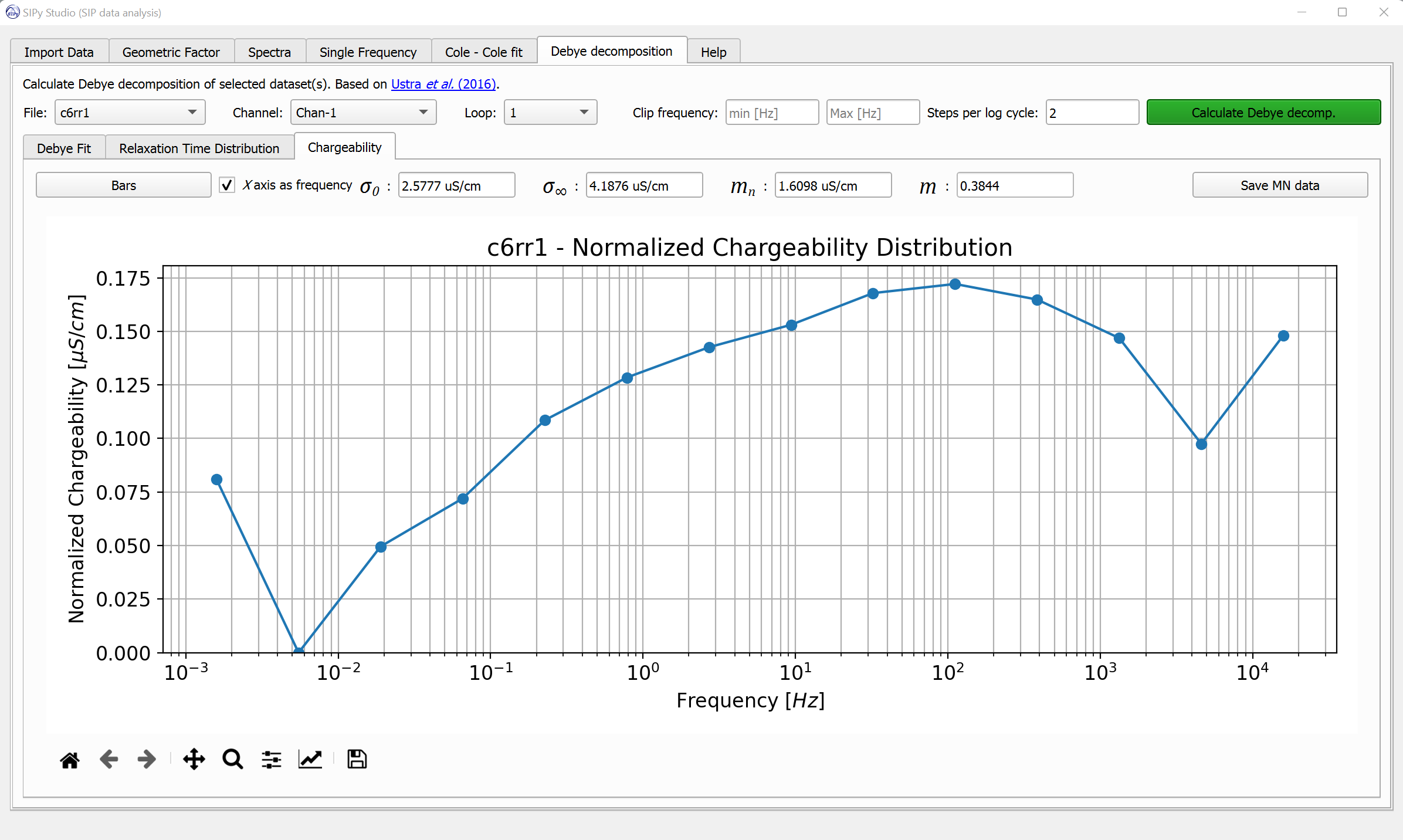
Precise Debye Decomposition Analysis

Debye decomposition inversion and calculation of relaxation time distribution with control on discretization steps included.

Graph showing relaxation time distribution with blue bars, titled 'c6rr1 - relaxation time distribution'. The x-axis is labeled 'Relaxation Time [s]' with a logarithmic scale from 10^-5 to 10^2 seconds, and the y-axis is labeled 'Relaxation time distribution (RTD)'.

Normalized Chargeability Calculations

Normalized chargeability distribution as well as total chargeability are calculated during Debye decomposition inversion.

Screenshot of a software interface showing a graph titled 'c6rr1 - Normalized Chargeability Distribution' with a plot of normalized chargeability versus frequency in Hz. The interface also contains controls and numerical data related to decibel decomposition analysis.

Please contact us for quotes and any questions on SIPy Studio data processing and visualization software

Quote

SIPy Studio

SIPy studio also offers the option to accurately calculate the geometric factor of experimental columns using conductivity and specific conductance of fluid solutions with known conductivity (the user can prepare them).

Trial Versions

You can download a fully featured trial version of SIPyStudio here:

for Windows

for MacOS, and

for Linux [Tested on Ubuntu]

The trial version is valid for 14 days. Upgrade to full licensed version does not require new installation (over the air upgrade).